Creating A Pie Chart In Microsoft Excel Tutorial With Pictures

Why Do We Use Excel Pie Charts?

Excel Pie Charts are used in a Microsoft Excel Worksheet to display the contribution of each cell value to the total value. Today, we will discuss the procedure of creating a Pie chart in Microsoft Excel. Start Microsoft Excel and perform the following steps as explained with the help of nice clear pictures.

Creating Excel Pie Charts Easy Tutorial With Pictures

Steps To Create Pie Chart in Excel

1. Prepare Example Excel Worksheet For Pie Chart

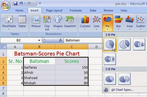
Start Microsoft Excel with a new blank workbook. Microsoft Excel is a part of Microsoft Office.
Prepare a new Excel Worksheet as shown in the figure below to show Serial Numbers, Batsman and their Scores got in a cricket match. Fill in the sample data as you wish.

2. Select Cell Range To Prepare Excel Pie Chart

Select The Two Columns named Batsman and Scores with filled values and column titles, as shown in the figure above.

3. Use Insert Tab To Create Pie Chart

Click on Insert Tab and click on Pie Chart tool. Select a suitable type of Pie Chart, say we select the very first type from 2D pie charts. When you will click on this type of pie chart, the Pie Chart will be crated and shown in the you Excel worksheet as shown below.

Steps to create a PIE Chart in MS Excel

Explain the use of Pie Charts in Excel spreadsheet software

4. Changing Layout of Excel Pie Chart

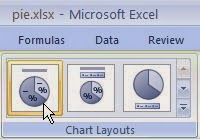
You can change the layout of your Pie chart easily by selecting a suitable layout on Chart Tools as shown in the figure below

5. Getting the Final Excel Pie Chart

As soon as you click on your selected layout, the Pie chart will be changed to new layout look as shown in the figure below.

Thank you for coming and staying with us at Www.ForFreeEducation.Blogspot.Com a totally free blog for  and much more.

You may also like to read:

Electricity Bill Calculator Formulas in Excel 

Using Simple Formulas in Excel With Arithmetic Operators 2